Dataless Physics Informed Neural Network (PINN) to Solve Laplace Equation using TensorFlow Keras in Python (Free Code)

     Here is code to solve 2D Laplace 🧨 equation using PINN🧠. This 👽 technology works with/without previous data. Soon I will add data loss using finite difference so to improve the neural network's accuracy. Soon 🤣. To convert this to 3D, add T_z and T_zz terms in laplace_equation and loss_fn functions.

import random as rn

import numpy as np

import matplotlib.pyplot as plt

import tensorflow as tf

from tensorflow import keras

from tensorflow.keras import layers

from tensorflow.keras.layers.experimental import preprocessing

# set same seeds for initialization

np.random.seed(0) # same random initializations every time numpy

rn.seed(0) # same random initializations every time for python 

tf.random.set_seed(0) # same random initializations every time for TensorFlow

# define the physics informed neural network structure

model = keras.Sequential([ # define a feedforward neural network with backpropagation and gradient descent with ADAM

    preprocessing.Normalization(input_shape=(2,)), # normalize inputs (2 for 2D, 3 for 3D)

    layers.Dense(50, activation='tanh', input_shape=(2, ), kernel_initializer='zeros'), # first hidden layer

    layers.Dense(50, activation='tanh'), # second hidden layer

    layers.Dense(1, activation=None) # output layer

])

# define the 2D Laplace equation and boundary conditions

def laplace_equation(le):

    with tf.GradientTape(persistent=True) as tape:

        tape.watch(le) # set the input variable le for gradient computation

        T = model(le) # predict the temperature field T using the neural network model

        T_x = tape.gradient(T, le)[:, 0]  # first derivative of neural network output with respect to x

        T_y = tape.gradient(T, le)[:, 1]  # first derivative of neural network output with respect to y

        T_xx = tape.gradient(T_x, le)[:, 0]  # second derivative of neural network output with respect to x

        T_yy = tape.gradient(T_y, le)[:, 1]  # second derivative of neural network output with respect to y

        eq_residual = T_xx + T_yy  # 2D Laplace equation: T_xx + T_yy = 0

        # apply boundary conditions

        left_bc = T[le[:, 0] == 0] - 0  # left boundary condition: T(x=0, y) = 0

        right_bc = T[le[:, 0] == 1] - 5  # right boundary condition: T(x=1, y) = 5

        top_bc = T[le[:, 1] == 1] - 20  # top boundary condition: T(x, y=1) = 20

        bottom_bc = T[le[:, 1] == 0] - 10  # bottom boundary condition: T(x, y=0) = 10

    return eq_residual, left_bc, right_bc, top_bc, bottom_bc

# define the loss function for 2D Laplace equation

def loss_fn(le):

    le = tf.convert_to_tensor(le, dtype=tf.float32) # convert le to TensorFlow tensor

    eq_residual, left_bc, right_bc, top_bc, \

        bottom_bc = laplace_equation(le)  # calculate the residuals and boundary conditions using the laplace_equation function

    mse_loss = tf.reduce_mean(tf.square(eq_residual)) # compute the mean squared error of the Laplace equation residuals

    bc_loss = tf.reduce_mean(tf.square(left_bc)) + tf.reduce_mean(tf.square(right_bc)) \

        + tf.reduce_mean(tf.square(top_bc)) + tf.reduce_mean(tf.square(bottom_bc)) # compute the mean squared error of the boundary conditions

    return mse_loss + bc_loss

# train the network

optimizer = tf.keras.optimizers.Adam(learning_rate=0.01) # specify learning rate and optimizer

max_epochs = 2000 # maximum iterations

epoch = 0 # iteration counter

loss_value = float('inf') # initial loss

min_loss = 0.01 # minimum loss (any acceptable value)

# generate sample points (grid)

L = 1 # length of the plate

D = 1 # width of the plate

Nx = 100 # number of points in x-axis

Ny = 100 # number of points in y-axis

train_points_x, train_points_y = np.meshgrid(np.linspace(0, L, Nx), np.linspace(0, D, Ny)) # create pairs of sample points along the domain

train_points = np.vstack((train_points_x.flatten(), train_points_y.flatten())).T # flatten the grid to feed to neural network

model.layers[0].adapt(train_points) # set up the normalization layer

# train the neural network

while epoch <= max_epochs and loss_value >= min_loss:

    with tf.GradientTape() as tape:

        loss_value = loss_fn(train_points)

    gradients = tape.gradient(loss_value, model.trainable_variables)

    optimizer.apply_gradients(zip(gradients, model.trainable_variables))

    epoch += 1 # increases iteration counter by 1

    if epoch % 100 == 0:

        print(f"Epoch {epoch}, Loss: {loss_value.numpy()}") # output loss while training

# prediction

test_points_x, test_points_y = np.meshgrid(np.linspace(0, L, Nx), np.linspace(0, D, Ny)) # create pairs of sample points along the domain (for testing)

test_points = np.vstack((test_points_x.flatten(), test_points_y.flatten())).T # flatten the grid to feed to neural network

predicted_temperature = model(test_points).numpy().reshape(test_points_x.shape) # neural network output

# plotting

plt.figure(dpi=600) # make nice crisp image :)

plt.contourf(test_points_x, test_points_y, predicted_temperature, cmap='turbo', levels=256) # contours of temperature

plt.colorbar(label='Temperature')

plt.xlabel('Length [m]')

plt.ylabel('Width [m]')

plt.title('2D Laplace Equation Solution using PINN')

plt.clim(0, 20) # Set legend limits

plt.show() # make plot

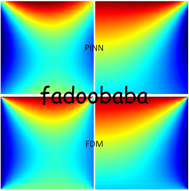
     Fig. 1, shows comparison with FDM using both Neumann and Dirichlet boundary conditions.  To apply Neumann boundary conditions, simply put T_x as 0 instead of T in the laplace_equation function. Within Fig. 1, right side is Dirichlet while Neumann is on the right side. Personally, FVM is still the king 👑.

Fig. 1, Top row PINN bottom row FDM

Update 01

     This new code has functions and handles the normalization of inputs manually. This version also has less derivatives to compute by some trickery, so it runs faster. Navier-Stokes version soon! I am not sure if PINN for Navier-Stokes equations go in CFD blog or in this blog? 😕 Also, this Update 1 code uses Keras 3 which is available on tensorflow-2.16.1.

#%% import stuff

import random as rn

import numpy as np

import matplotlib.pyplot as plt

import tensorflow as tf

import keras

from keras import layers

#%% define the 2D Laplace equation and boundary conditions

def laplace_equation(le):

    with tf.GradientTape(persistent=True) as tape2:

        tape2.watch(le) # watch the input variable le for 2nd order gradient computation

        

        with tf.GradientTape(persistent=True) as tape1:

            tape1.watch(le) # set the input variable le for 1st order gradient computation

            

            T = model(le) # predict the temperature field T using the neural network model

        

        dT = tape1.gradient(T, le) # dT/dle

        T_x = dT[:, 0] # d2T/dx2

        T_y = dT[:, 1] # d2T/dy2

        

    T_xx = tape2.gradient(T_x, le)[:, 0] # d2T/dx2

    T_yy = tape2.gradient(T_y, le)[:, 1] # d2T/dy2

    eq_residual = T_xx + T_yy # 2D Laplace equation: T_xx + T_yy = 0

        

    # apply boundary conditions

    left_bc = T[le[:, 0] == 0] - 0 # left boundary condition: T(x = 0, y) = 0

    right_bc = T_x[le[:, 0] == 1] - 0 # right boundary condition: dT/dx(x = L, y) = 0

    top_bc = T[le[:, 1] == 1] - 1 # top boundary condition: T(x, y = 1) = 1

    bottom_bc = T_y[le[:, 1] == 0] - 0 # bottom boundary condition: dT/dy(x, y = 0) = 0

    return eq_residual, left_bc, right_bc, top_bc, bottom_bc

#%% define the loss function for 2D Laplace equation

def loss_fn(le):

    le = tf.convert_to_tensor(le, dtype=tf.float32) # convert le to TensorFlow tensor

    eq_residual, left_bc, right_bc, top_bc,\

        bottom_bc = laplace_equation(le) # calculate the residuals and boundary conditions using the laplace_equation function

    

    mse_loss = tf.reduce_mean(tf.square(eq_residual)) # compute the mean squared error of the Laplace equation residuals

    

    bc_loss = tf.reduce_mean(tf.square(left_bc)) + tf.reduce_mean(tf.square(right_bc)) \

        + tf.reduce_mean(tf.square(top_bc)) + tf.reduce_mean(tf.square(bottom_bc)) # compute the mean squared error of the boundary conditions

    

    total_loss = mse_loss + bc_loss # total loss

    

    return total_loss

#%% set same seeds for initialization

np.random.seed(42) # same random initializations every time numpy

rn.seed(42) # same random initializations every time for python 

tf.random.set_seed(42) # same random initializations every time for TensorFlow / Keras

#%% generate sample points (grid)

L = 3.25 # length of the plate

D = 2.75 # width of the plate

Nx = 20 # number of points in x-axis

Ny = 20 # number of points in y-axis

x = np.linspace(0, L, Nx) # mesh in x axis

y = np.linspace(0, D, Ny) # mesh in y axis

x = x / L # normalize x

y = y / D # normalize y

#%% create the neural network

model = keras.Sequential([layers.Input(shape=(2,)), # input layer, 2 for x and y

                          layers.Dense(20, activation = 'tanh', kernel_initializer='GlorotNormal', bias_initializer='zeros'), # hidden layer

                          layers.Dense(1, activation = None)]) # output layer, 1 for T

model.summary() # display model

#%% define the physics informed neural network structure

train_points_x, train_points_y = np.meshgrid(x, y) # create pairs of sample points along the domain

train_points = np.vstack((train_points_x.flatten(), train_points_y.flatten())).T # flatten the grid to feed to neural network

optimizer = tf.keras.optimizers.Adam() # specify learning rate and optimizer

max_epochs = 10000 # maximum iterations

for epoch in range(1, max_epochs + 1): # training loop

    with tf.GradientTape() as tape3:

        loss_value = loss_fn(train_points) # compute total loss by evaluating Navier-Stokes loss function on training points

    gradients = tape3.gradient(loss_value, model.trainable_variables) # calculate gradients of total loss with respect to trainable variables of model

    optimizer.apply_gradients(zip(gradients, model.trainable_variables)) # update model trainable variables using calculated gradients and specified optimizer

    epoch += 1  # increases iteration counter by 1

    if epoch % 100 == 0:

        # print(f"Epoch {epoch}")

        print(f"Epoch {epoch}, Loss: {loss_value.numpy()}")

#%% prediction

x_t = np.linspace(0, L, 10)  # initialize x

y_t = np.linspace(0, D, 10)  # initialize y

x_t = x_t / L # notmalize test data x-axis

y_t = y_t / D # notmalize test data y-axis

test_points_x, test_points_y = np.meshgrid(x_t, y_t)  # create pairs of sample points along the domain (for testing)

test_points = np.vstack((test_points_x.flatten(), test_points_y.flatten())).T  # flatten the grid to feed to the neural network model

predict = model.predict(test_points) # predict temperature

# plotting

plt.figure(dpi = 300) # make nice crisp image

plt.contourf(test_points_x * L, test_points_y * D, predict.reshape(test_points_x.shape), cmap = 'jet', levels = 32) # contours of temperature

plt.colorbar(orientation='vertical')

plt.clim(0, 1) # set legend limits

plt.axis("equal")

plt.show() # show plot

     If you want to hire me as your PhD student or collaborate in cutting-edge research, please reach out!